Lab 14: Classification I: Prediction and Probability Calibration

For the class on Monday, March 25th

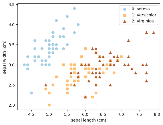
We use the Iris data set in this lab to demonstrate a few classification methods and related techniques.

Because we are using the data set only as a demonstration, we will use all data as training data, but be aware that this is not a good practice when you have a real problem to tackle!

We also only use two of the four available features so that it is easier to visualize. This again is not what you typically want to do when analyzing a real problem.

import matplotlib.pyplot as plt
from sklearn import datasets
from sklearn.naive_bayes import GaussianNB
from sklearn.neighbors import KNeighborsClassifier
from sklearn.gaussian_process import GaussianProcessClassifier
from sklearn.calibration import CalibratedClassifierCV
from sklearn.inspection import DecisionBoundaryDisplay
from sklearn.metrics import ConfusionMatrixDisplay
from sklearn.calibration import CalibrationDisplay

# Load the iris data
iris = datasets.load_iris()
X = iris.data[:, :2]  # we only take the first two features.
Y = iris.target

# Plot the iris data
n_classes = len(iris.target_names)
for i in range(n_classes):
    plt.scatter(X[Y==i, 0], X[Y==i, 1], color=plt.cm.Paired(i/(n_classes-1)), marker="os^"[i], label=f"{i}: {iris.target_names[i]}")
plt.legend()
plt.xlabel(iris.feature_names[0])
plt.ylabel(iris.feature_names[1]);

A. Decision boundaries, classification probability, confusion matrix

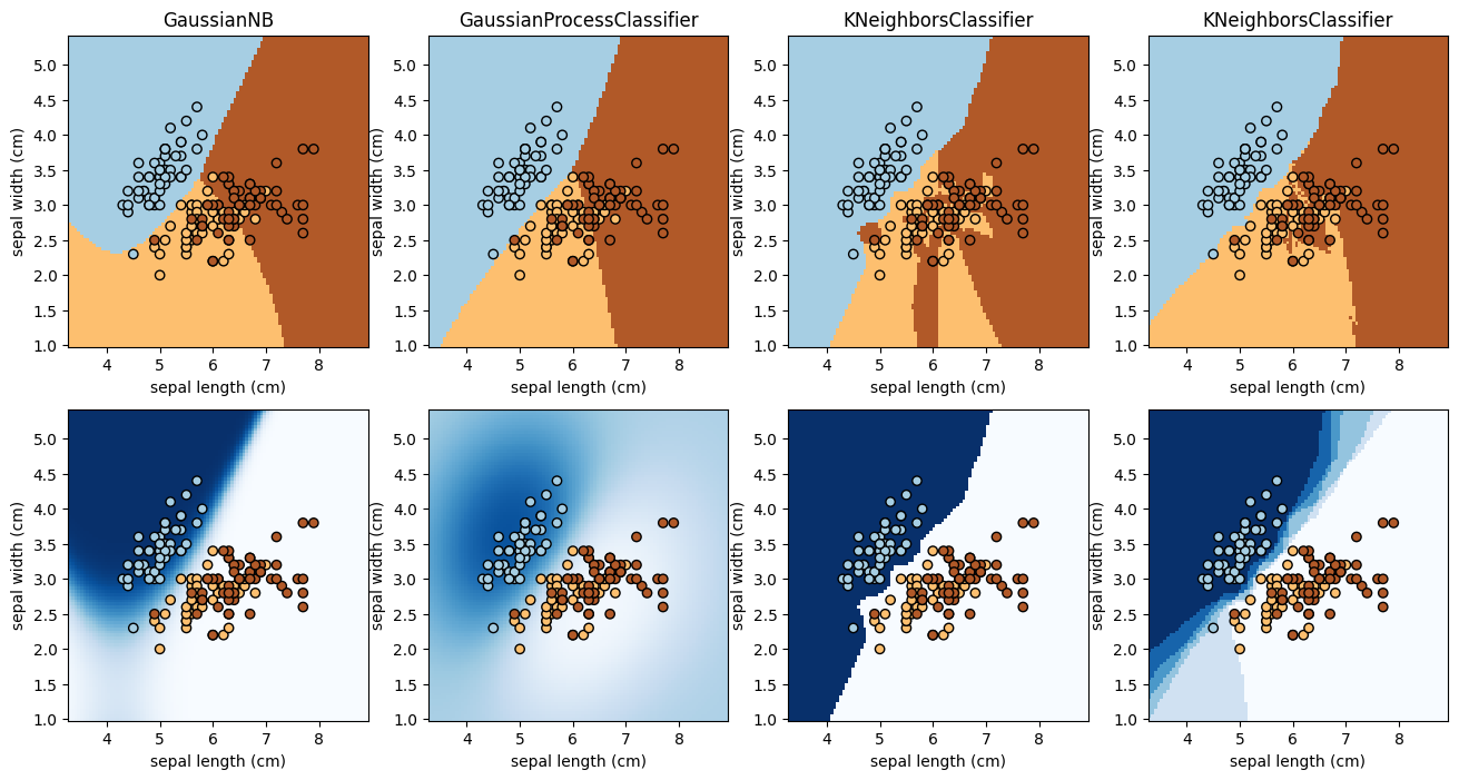
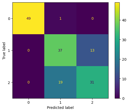
We will test four different classifiers on the Iris data set, and plot their decision boundaries in the feature space. We will also show the classification probability for Class 0 (Setosa) for each method. Finally we plot the confusion matrix for all 3 classes for the Naive Bayes method.

# Code modified from https://scikit-learn.org/stable/auto_examples/linear_model/plot_iris_logistic.html

classifiers = [
    GaussianNB(),
    GaussianProcessClassifier(),
    KNeighborsClassifier(n_neighbors=1),
    KNeighborsClassifier(n_neighbors=5),
]

fig, ax = plt.subplots(2, 4, figsize=(16,8))

for i, clf in enumerate(classifiers):
    clf.fit(X, Y)

    DecisionBoundaryDisplay.from_estimator(
        clf,
        X,
        cmap=plt.cm.Paired,
        ax=ax[0,i],
        response_method="predict",
        plot_method="pcolormesh",
        shading="auto",
        xlabel=iris.feature_names[0],
        ylabel=iris.feature_names[1],
    )

    DecisionBoundaryDisplay.from_estimator(
        clf,
        X,
        cmap=plt.cm.Blues,
        ax=ax[1,i],
        response_method="predict_proba",
        class_of_interest=0,
        plot_method="pcolormesh",
        shading="auto",
        xlabel=iris.feature_names[0],
        ylabel=iris.feature_names[1],
        vmin=0,
        vmax=1,
    )

    # Plot also the training points
    for j in [0, 1]:
        ax[j,i].scatter(X[:, 0], X[:, 1], c=Y, edgecolors="k", cmap=plt.cm.Paired)

    ax[0,i].set_title(clf.__class__.__name__)

# Confusion matrix
clf = GaussianNB()
clf.fit(X, Y)
ConfusionMatrixDisplay.from_estimator(clf, X, Y);

Part A Questions:

1. The lower panels of the first plot show the classification probability. Note that for the KNeighborsClassifier, the shades (which show the probability for Class 0) are discrete. There are two and six shades respectively for the two different KNeighborsClassifier setups (with different n_neighbors values). Explain where the number of shades you observed comes from.

2. What value of probability do the decision boundaries correspond to?

3. If you see an iris with a sepal length of 4 cm and a sepal width of 5 cm, which class would you predict? Is your prediction consistent with the four methods?

4. Continued with (2), how confident is your prediction? Is your confidence consistent with the four methods? Which of the four methods gives the most different result? Can you explain why?

5. Based on the confusion matrix: (a) what is the recall for Class 1? (b) what is the contamination for Class 2? Write down the formula you use to do the calculation.

---

// Write your answer here

---

B. Probability Calibration

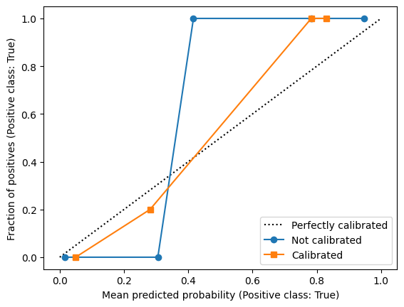
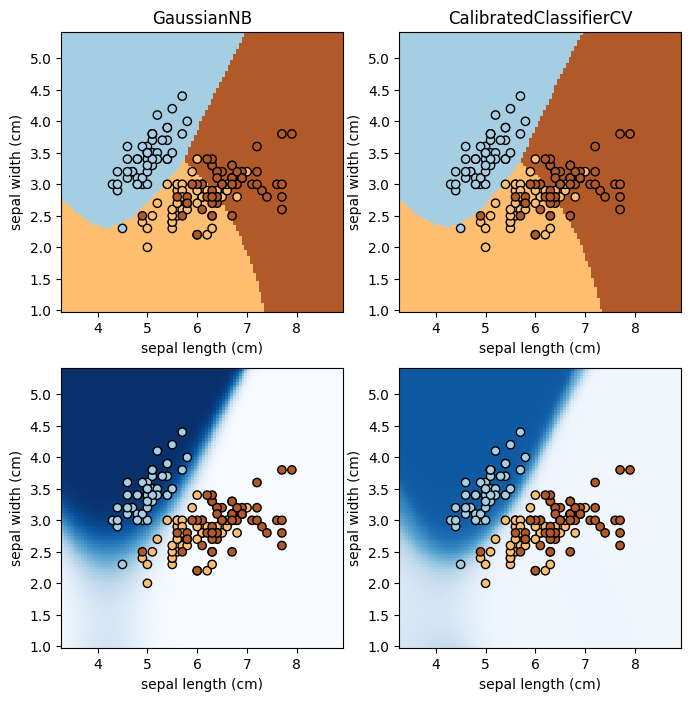
Here we apply the probability calibration to the Gaussian Naive Bayes classifier.

We first show the calibration plot, and then show the decision boundaries and probability map (for Class 0). In all 3 plots we show both the uncalibrated and calibrated classifiers.

classifiers = [
    GaussianNB(),
    CalibratedClassifierCV(GaussianNB()),
]

fig, ax = plt.subplots()
class_index = 0
for i, clf in enumerate(classifiers):
    clf.fit(X, Y)

    CalibrationDisplay.from_predictions(
        (Y == class_index),
        clf.predict_proba(X)[:,class_index],
        ax=ax,
        n_bins=5,
        pos_label=True,
        name=("Calibrated" if i else "Not calibrated"),
        marker=("s" if i else "o"),
    )

classifiers = [
    GaussianNB(),
    CalibratedClassifierCV(GaussianNB()),
]

fig, ax = plt.subplots(2, 2, figsize=(8,8))

for i, clf in enumerate(classifiers):
    clf.fit(X, Y)

    DecisionBoundaryDisplay.from_estimator(
        clf,
        X,
        cmap=plt.cm.Paired,
        ax=ax[0,i],
        response_method="predict",
        plot_method="pcolormesh",
        shading="auto",
        xlabel=iris.feature_names[0],
        ylabel=iris.feature_names[1],
    )

    DecisionBoundaryDisplay.from_estimator(
        clf,
        X,
        cmap=plt.cm.Blues,
        ax=ax[1,i],
        response_method="predict_proba",
        class_of_interest=0,
        plot_method="pcolormesh",
        shading="auto",
        xlabel=iris.feature_names[0],
        ylabel=iris.feature_names[1],
        vmin=0,
        vmax=1,
    )

    for j in [0,1]:
        ax[j,i].scatter(X[:, 0], X[:, 1], c=Y, edgecolors="k", cmap=plt.cm.Paired)
    ax[0,i].set_title(clf.__class__.__name__)

Part B Questions:

1. Explain how the calibration plot was made. For example, there is a blue point around \((x=0.3, y=0)\). How was the location of that point calculated? (In other words, you should be able to make this plot without using CalibrationDisplay, even though you are not asked to actually implement it here.)

2. Does the probability calibration affect the decision boundaries? If so, in what way does it affect them?

3. Does the probability calibration affect the probability map? If so, in what way does it affect the map?

4. Do you think the probability calibration was robust in this case? Try changing the n_bins value in CalibrationDisplay.from_predictions to test. If not, what may be the main factor that prohibits a good calibration?

---

// Write your answer here

---

Tip

How to submit this notebook on Canvas?

1. Make sure all your answers, code, and desired results are properly displayed in the notebook.

2. Save the notebook (press Ctrl+s or Cmd+s). The grey dot on the filename tab (indicating “unsaved”) should disappear.

3. Run the following cell.

4. Upload the resulting HTML file to Canvas under the corresponding assignment.

! jupyter nbconvert --to html ./14.ipynb