Lab 13: Regression II: Gaussian Process and Cross Validation

For the class on Monday, March 17th

import numpy as np
import matplotlib.pyplot as plt
import pandas as pd

from sklearn.model_selection import train_test_split
from sklearn.linear_model import LinearRegression, LogisticRegression
from sklearn.gaussian_process import GaussianProcessRegressor
from sklearn.model_selection import cross_val_score, GridSearchCV

A. Gaussian Process Regression

In this example, we have a simple data set with only one feature and one target. A simple linear regression does not fit this data set. We will test if Gaussian Process regression works well in this case.

A1. Compare Gaussian Process and Linear Regression

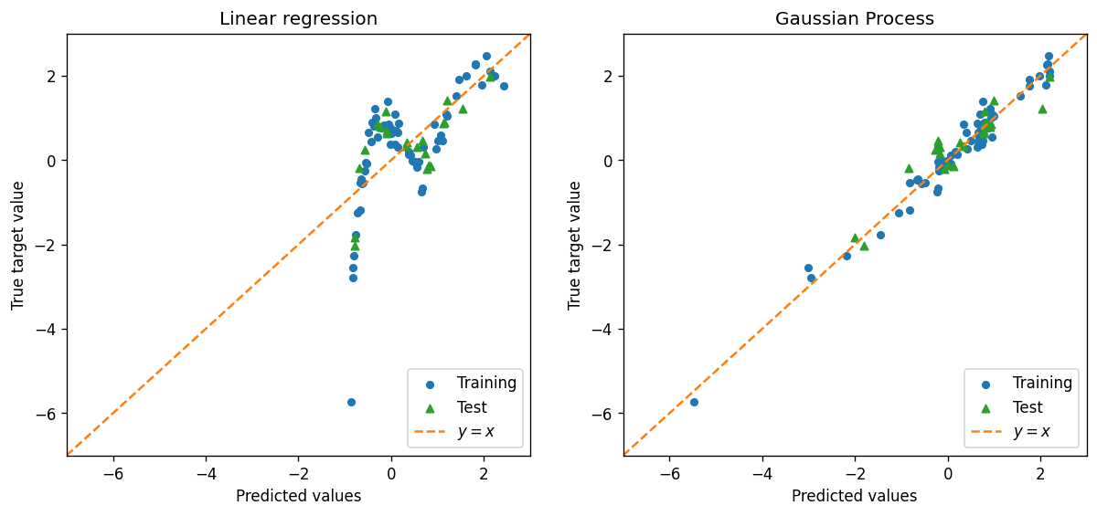
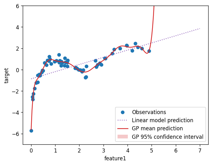
Here we will compare the performance of Gaussian Process regression and linear regression on the data set. The first plot shows the predicted target value vs. the actual target value for both the training and test sets. The second plot shows the target value vs. the feature value for the training set.

df = pd.read_csv("https://yymao.github.io/phys7730/lab13a.csv")
df.head()

	feature1	target
0	1.790917	0.411666
1	0.351093	-0.555546
2	0.755384	1.215104
3	0.923896	0.793547
4	0.275408	-1.181132

train_features, test_features, train_target, test_target = train_test_split(df[["feature1"]], df["target"], test_size=0.25, random_state=456)

# Note that, despite the difference between `reg_lr` and `reg_gp`,
# The code to fit the data and make prediction is almost identical.

reg_lr = LinearRegression()
reg_lr.fit(train_features, train_target)
train_predict_lr = reg_lr.predict(train_features)
test_predict_lr = reg_lr.predict(test_features)

reg_gp = GaussianProcessRegressor(normalize_y=True)
reg_gp.fit(train_features, train_target)
train_predict_gp = reg_gp.predict(train_features)
test_predict_gp = reg_gp.predict(test_features)

fig, ax = plt.subplots(ncols=2, figsize=(12, 5), dpi=120)

ax[0].scatter(train_predict_lr, train_target, c="C0", s=20, label="Training")
ax[0].scatter(test_predict_lr, test_target, c="C2", s=25, marker="^", label="Test")
ax[0].set_title("Linear regression")

ax[1].scatter(train_predict_gp, train_target, c="C0", s=20, label="Training")
ax[1].scatter(test_predict_gp, test_target, c="C2", s=25, marker="^", label="Test")
ax[1].set_title("Gaussian Process")

corners = [-7, 3]
for ax_this in ax:
    ax_this.plot(corners, corners, c="C1", ls="--", label="$y=x$")
    ax_this.set_xlim(*corners)
    ax_this.set_ylim(*corners)

    ax_this.set_xlabel("Predicted values")
    ax_this.set_ylabel("True target value")
    ax_this.legend(loc="lower right");

x = np.linspace(0, 7, 201)
prediction_lr = reg_lr.predict(pd.DataFrame({"feature1": x}))
mean_prediction_gp, std_prediction_gp = reg_gp.predict(pd.DataFrame({"feature1": x}), return_std=True)

fig, ax = plt.subplots(dpi=120)
ax.scatter(train_features["feature1"], train_target, label="Observations")
ax.plot(x, prediction_lr, label="Linear model prediction", ls=":", c="C4")
ax.plot(x, mean_prediction_gp, label="GP mean prediction", c="C3")
ax.fill_between(
    x.ravel(),
    mean_prediction_gp - 1.96 * std_prediction_gp,
    mean_prediction_gp + 1.96 * std_prediction_gp,
    alpha=0.25,
    color="C3",
    label=r"GP 95% confidence interval",
    lw=0,
)
ax.legend(loc="lower right")

ax.set_ylim(-7, 6)
ax.set_xlabel("feature1")
ax.set_ylabel("target");

📝 Questions (Part A1):

1. Based on the first plot, how would you compare the performance of the linear regression and the Gaussian Process regression?

2. Based on the second plot, does your evaluation of the two methods (linear regression and the Gaussian Process regression) change? Briefly explain why.

3. Why don’t we see the GP 95% confidence interval on the second plot?

4. Which method do you think would give a better prediction when the feature1 value is around 1? Why?

5. Which method do you think would give a better prediction when the feature1 value is around 7? Why?

// Write your answers to Part A1 here

A2. Including data uncertainty

🚀 Tasks

1. Repeat Part A1 (including making those plots), but change GaussianProcessRegressor(normalize_y=True) to GaussianProcessRegressor(normalize_y=True, alpha=0.1).

   Tip

   What is alpha? Roughly speaking, it’s the assumed uncertainty of data points (in target). See the documentation of GaussianProcessRegressor for detail.

2. Manually try a few different values of alpha (no need to refactor or optimize your code, as you’ll see a better way in Part B). What value seems to give you the best result?

# Add your implementation to A2 here.

📝 Questions (Part A2):

1. During Step 2, what value of alpha seems to work well? How did you define “work well”?

// Write your answers to Part A2 here

B. Cross Validation

In Part B, we will use cross validation to find the optimal values for the hyperparameter in our ML models.

B1. Gaussian Process

cross_val_score(GaussianProcessRegressor(normalize_y=True), train_features, train_target)

array([ 0.94466647,  0.8790451 ,  0.91188481, -7.1283826 ,  0.72405611])

reg_cv = GridSearchCV(GaussianProcessRegressor(normalize_y=True), {"alpha": np.logspace(-8, 1, 31)})
reg_cv.fit(train_features, train_target);

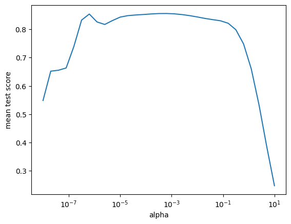
plt.semilogx(reg_cv.cv_results_["param_alpha"].data, reg_cv.cv_results_["mean_test_score"])
plt.xlabel("alpha")
plt.ylabel("mean test score");

📝 Questions (Part B1):

1. The first cell (right below the B1 heading) has an output of 5 numbers. What do these numbers mean? And why are there five numbers (but not four or six)? (Hint: Check out the documentation of cross_val_score.)

2. Based on the plot right above, what value of alpha gives the Gaussian Process model the best performance on this data set? Is this value similar to what you found in Part A2?

// Write your answers to Part B1 here

B2. Revisit Lab 12 Part B

In Lab 12 Part B, we compare the logistic regression method with and without regularization. When regularization is included (the default option for LogisticRegression), we can in fact further adjust the regularization strength by changing the value supplied to the argument C. See the documentation of LogisticRegression for details.

In this part, we will use the cross validation method we just learned to justify our discussion in Lab 12 Part B.

df_12b = pd.read_csv("https://yymao.github.io/phys7730/lab12b.csv")
train_12b_features, test_12b_features, train_12b_target, test_12b_target = train_test_split(df_12b.iloc[:,:3], df_12b["target"], test_size=0.25, random_state=123)

reg_cv = GridSearchCV(LogisticRegression(), {"C": np.logspace(-3, 3, 31)})
reg_cv.fit(train_12b_features, train_12b_target);

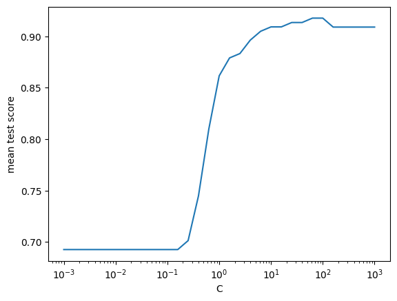
plt.semilogx(reg_cv.cv_results_["param_C"].data, reg_cv.cv_results_["mean_test_score"])
plt.xlabel("C")
plt.ylabel("mean test score");

📝 Questions (Part B2):

1. Based on the plot above, do you think including regularization is helpful for this particular data set?

2. Note that your answer to Q1 is not a general statement about regularization! What do you think is special about this data set that results in your conclusion?

// Write your answers to Part B2 here

Tip

Submit your notebook

Follow these steps when you complete this lab and are ready to submit your work to Canvas:

1. Check that all your text answers, plots, and code are all properly displayed in this notebook.

2. Run the cell below.

3. Download the resulting HTML file 13.html and then upload it to the corresponding assignment on Canvas.

!jupyter nbconvert --to html --embed-images 13.ipynb