Lab 7: Ising Model#
For the class on Wednesday, February 5th
Code for simulating a 2D Ising Model#
The following cell defines the IsingModel2D class, which implements a numerical
representation of a 2D Ising Model and the associated MCMC simulation methods.
You need to run this cell, but you don’t need to edit anything in it. You are welcome to take a look at the code of the class, but it is not necessary to understand the code in detail to complete the lab.
Show code cell source
import numpy as np
import matplotlib.pyplot as plt

class IsingModel2D:
    def __init__(self, side_length: int, boundaries=None, initial_values="cold", antiferro=False):
        self._side_length = int(side_length)
        self._size = self._side_length * self._side_length

        indices = np.arange(self._size).reshape((self._side_length, self._side_length))
        neighbor_indices = np.stack([
            np.roll(indices, 1, 0),   # up
            np.roll(indices, -1, 1),  # right
            np.roll(indices, -1, 0),  # down
            np.roll(indices, 1, 1),   # left
        ])

        if boundaries not in [None, "periodic"]:
            try:
                bu, br, bd, bl = boundaries
            except TypeError:
                bu = br = bd = bl = boundaries
            idx = np.arange(self._size, self._size + 3)
            for bv, s in zip([bu, br, bd, bl], [(0,0), (1,Ellipsis,-1), (2,-1), (3,Ellipsis,0)]):
                neighbor_indices[s] = idx[int(np.sign(bv))]

        self._neighbor_indices = neighbor_indices.reshape(4, self._size).T

        self._data = np.empty(self._size + 3, dtype=np.int32)
        self._data[-3:] = [0, 1, -1]
        if isinstance(initial_values, str):
            if initial_values == "hot":
                self.data = np.random.default_rng().random(self._size) >= 0.5
            elif initial_values == "cold":
                self.data = 1
        else:
            self.data = initial_values

        self._J = float(-1 if antiferro else 1)

    @property
    def size(self):
        return self._size

    @property
    def data(self):
        return self._data[:-3].reshape(self._side_length, self._side_length).copy()

    @data.setter
    def data(self, value):
        value = np.ravel(value)
        if len(value) not in [1, self._size]:
            raise ValueError(f"`value` must be a single value or an array of size {self._size}")
        new_value = np.ones(len(value), dtype=np.int32)
        new_value[~(value > 0)] = -1
        if len(new_value) == 1:
            new_value = new_value[0]
        self._data[:-3] = new_value

    def show(self, **kwargs):
        plt.matshow(self.data, vmax=1, vmin=-1, **kwargs)

    def _check_site_index(self, site_index: int):
        if not isinstance(site_index, int):
            i, j = site_index
            site_index = int(i) * self._side_length + int(j)
        if site_index >= 0 and site_index < self._size:
            return site_index
        raise ValueError(f"`site_index` must be between 0 and {self._size - 1} (inclusive)")

    def calc_magnetization(self):
        return self._data[:self._size].sum(dtype=np.float64) / self._size

    def calc_total_energy(self, ext_field=0.0):
        energy = (
            self._data[self._neighbor_indices].sum(axis=1, dtype=np.float64)
            * self._data[:self._size]
        ).sum(dtype=np.float64) * self._J * (-0.5)
        if ext_field:
            energy -= self._data[:self._size].sum(dtype=np.float64) * float(ext_field)
        return energy

    def calc_local_energy(self, site_index: int, ext_field=0.0):
        site_index = self._check_site_index(site_index)
        energy = (
            self._data[self._neighbor_indices[site_index]].sum(dtype=np.float64)
            * self._data[site_index]
            * self._J
            * (-1.0)
        )
        if ext_field:
            energy -= self._data[site_index] * float(ext_field)
        return energy

    def flip(self, site_index):
        self._data[self._check_site_index(site_index)] *= -1

    def transition_prob_metropolis(self, site_index: int, beta: float, ext_field=0.0):
        return np.exp(2.0 * beta * self.calc_local_energy(site_index, ext_field))

    def transition_prob_gibbs(self, site_index: int, beta: float, ext_field=0.0):
        return 1.0 / (1.0 + np.exp(-2.0 * beta * self.calc_local_energy(site_index, ext_field)))

    def sweep(self, beta, ext_field=0.0, nsweeps=1, seed=None, transition_prob="metropolis"):
        rng = np.random.default_rng(seed)
        transition_prob_func = getattr(self, f"transition_prob_{transition_prob}")
        accept = 0
        for _  in range(nsweeps):
            for i in range(self._size):
                if rng.random() < transition_prob_func(i, beta, ext_field):
                    self.flip(i)
                    accept += 1
        return accept / self._size / nsweeps
A. Energy and Magnetization Calculations#
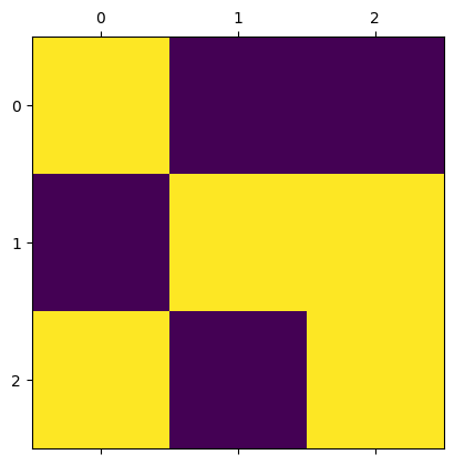
The following cell shows a 3-by-3 two-dimensional Ising model with a specific initial condition.
The yellow/light color in the image represents a spin of \(+1\), and the purple/dark color represents a spin of \(-1\).
📝 Questions:
Calculate the average magnetization \(\frac{1}{N} \sum_i \sigma_i\).
Calculate the energy from pairs associated with the central cell [with indices (1,1)]:
\[ - \sum_{j \in D} \sigma_i \sigma_j \text{, where } i=(1,1) \text{ and } D = \text{neighbors of } i \]If the spin of the central cell flips from \(+1\) to \(-1\), how much will the total energy of the system change?
How do your answers to (2) and (3) relate to each other? Briefly explain.
Verify your answers with the code below. Does the result agree with your calculations?
// Add your answers to Part A here
# Do not edit this cell
m = IsingModel2D(side_length=3, initial_values=[1,-1,-1,-1,1,1,1,-1,1])
m.show()
# Uncomment and run the following codes to verify your answers

#print("1. Average magnetization:", m.calc_magnetization())

#print("2. Local energy of site (1,1):", m.calc_local_energy(site_index=(1,1)))

#print("3. Total energy before flip:", m.calc_total_energy())
#m.flip(site_index=(1,1))
#print("3. Total energy after flip:", m.calc_total_energy())
B. Critical Temperature#
Let’s first take a look at how the sweep method works.
When calling sweep, the argument beta sets the temperature of the system with \(\beta = 1/kT\).
The argument nsweeps sets the number of sweeps to perform. Each sweep updates all sites in the lattice once.
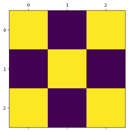
m = IsingModel2D(side_length=3, initial_values="hot")
m.show()
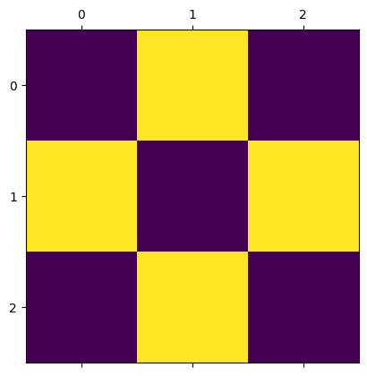
m.sweep(beta=0.3, nsweeps=1)
m.show()
We will run a simulation and gradually lower the temperature, in order to observe how the magnetization changes with temperature.
🚀 Tasks and Questions:
Set up a 25-by-25 lattice with the “hot” initial condition.
We will vary
beta(\(\beta = 1/kT\)) from 0.1 to 0.9, with a step of 0.02.For each value of
beta, we will run 20 “sweeps”.We will measure the average magnetization (averaged over sites) for each value of
beta, after the 20 sweeps ran.Make a plot of the average magnetization as a function of
beta(\(m\)-\(\beta\) relation).Describe what you observe. Does the magnetization show a sudden change at a certain value of \(\beta\)?
# Complete "..." in the the follow code
from tqdm.notebook import tqdm

m = IsingModel2D(...)

beta_values = np.arange(0.1, 0.91, 0.02)
magnetization_values = []

for beta in tqdm(beta_values):
    m.sweep(...)
    magnetization_values.append(m.calc_magnetization())
fig, ax = plt.subplots(dpi=150)
ax.plot(beta_values, magnetization_values)
ax.grid(True)
ax.set_xlabel("$\\beta = 1/kT$")
ax.set_ylabel("$\\langle m \\rangle$ Average magnetization")
// Write your answers to Part B here
C. Your Experiment!#
🚀 Tasks and Questions:
Choose at least one of the following conditions to experiment. Observe how the \(m\)-\(\beta\) relation changes:
as the external field strength changes (choose a few values from 0 to 2; set
ext_fieldwhensweepis called);as the lattice size changes (choose a few numbers between 5 and 100; set
side_lengthwhen setting up the model); oras the boundary condition changes (try
1,-1,[1,1,-1,-1],[1,-1,1,-1]; setboundarieswhen setting up the model)
and describe what you observe.
Use the earlier example as a reference to for how to implement you experiment. If you have time, you are welcome to do more than one experiment, or come up with your own ideas.
# Include your implementation for Part C here
// Write your answers to Part C here
Tip
Submit your notebook
Follow these steps when you complete this lab and are ready to submit your work to Canvas:
Check that all your text answers, plots, and code are all properly displayed in this notebook.
Run the cell below.
Download the resulting HTML file
07.htmland then upload it to the corresponding assignment on Canvas.
!jupyter nbconvert --to html --embed-images 07.ipynb