Lab 6: Random walk and Brownian motion

For the class on Wednesday, January 31st

You can answer the questions based on the discussion you had with your partner in class. (Indicate your partner’s name if applicable.)

Tip

Looking for hints?

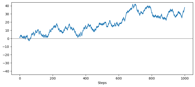
Demo: One path of a simple random walk

Here we are showing a simple random walk, \(x_N = \sum_{i=1}^{N} s_i\), where \(s_i\) is sampled uniformly from \(\{1,-1\}\).

Each time you rerun the cell below you will see a differnet path of a 1000-step simple random walk.

import numpy as np
import matplotlib.pyplot as plt

n_steps_total = 1000
s = np.random.default_rng().integers(2, size=n_steps_total) * 2 - 1
x = np.cumsum(s)

plt.figure(figsize=(10,4))
plt.plot(np.arange(n_steps_total), x);
plt.axhline(0, c="grey", lw=1);
lim = np.max(np.abs(plt.gca().get_ylim()))
plt.ylim(-lim, lim);
plt.xlabel("Steps");

A. Scaling and convergence of the diffusively rescaled random walk

Recall from Reading 6, the diffusively rescaled random walk is defined as

\[ W_N(t) = \frac{x_{\lfloor Nt \rfloor}}{\sqrt{N}}. \]

Questions

1. What is the variance of \(x_N\)? Verify your answer with the implementation below.

2. What is the variance of \(W_N(1)\)? Verify your answer with implementation below.

3. Write down an example of how you would check that the diffusively rescaled random walk \(W_N(t)\) converges as \(N\) increases.

---

// Add your answers to A here

---

Steps for Implementation

Here we will implement the diffusively rescaled random walk defined in Reading 06.

Here’s the setup of this random walk:

• Runs from \(t=0\) to \(t=1\).

• Each unit of time time discretized to \(N\) steps. We will start with \(N=100\).

Here’s the steps to generate multiple realization of this random walk:

1. Calculate the total number of steps \(Nt_\text{max}\) you need. Store that in n_steps_total.

2. Generate the increments at the steps \(s_i\) for one diffusively rescaled random walk (see demo above)

3. Calculate the paths \(x_k = \sum_{i=0}^{k} s_i\) of this particular random walk (use np.cumsum; see demo above).

4. Repeat [Steps 2 and 3] for \(n_\text{path} = 10,000\) times.

5. Plot the quantile function of \(W_N(t) = x_{\lfloor Nt \rfloor} / \sqrt{N}\) at \(t=1\).

Now, repeat this whole process with a few choices of \(N\) (e.g., 100, 1,000, 10,000), and then check:

• The variances of \(x_N\) and \(W_N(1)\).

• Does the cumulative distribution function of \(W_N(t=1)\) look like a standard normal distribution regardless of the value of \(N\)?

• As \(N\) increases, does the cumulative distribution function look more like a standard normal distribution?

# Include your implementation for Part A here

B. Universality of simple random walks

Questions

Based on the Central Limit Theorem (CLT), if the increments at individal steps are not sampled uniformly from \(\{1,-1\}\), but from a continuous uniform distribution \(\mathcal{U}(-1, 1)\), how would the distribution of \(W_N(t=1)\) look like as \(n \to\infty\)?

---

// Add your answers to Part B here

---

Steps for Implementation

Copy the implementation from Part A, and then change the distribution from which \(s_i\) is sampled to \( s_i \sim \mathcal{U}(-1, 1)\) (continuous uniform distribution on \([-1, 1]\)).

Calculate the cumulative distribution function \(W_{N=100}(t=1)\) in this case, and then check:

• Does it look like a standard normal distribution?

• If not, what distribution does it look like? Can you make it look like a standard normal distribution?

# Include your implementation for Part B here

Final question

Roughly how much time did you spend on this lab (not including the time you spent in class)?

---

// Write your answers here

---

Tip

How to submit this notebook on Canvas?

Once you complete this lab and have all your code, text answers, and all the desired results after running the notebook properly displayed in this notebook, please convert the notebook into HTML format by running the following:

jupyter nbconvert --to html /path/to/labs/06.ipynb 

Then, upload the resulting HTML file to Canvas for the corresponding assignment.