Lab 15: Classification II: Decision Trees and Ensemble Methods#
For the class on Wednesday, March 27th
A. Comparing Classification Methods#
This plot that compares different classification methods was shown in class when we discussed how the predicted “probability” is calculated by each method.
Document your discussion in class below.
Show code cell source
# Modified from https://scikit-learn.org/stable/auto_examples/classification/plot_classifier_comparison.html

import matplotlib.pyplot as plt
import numpy as np
from matplotlib.colors import ListedColormap

from sklearn.datasets import make_circles, make_classification, make_moons
from sklearn.discriminant_analysis import QuadraticDiscriminantAnalysis
from sklearn.gaussian_process import GaussianProcessClassifier
from sklearn.gaussian_process.kernels import RBF
from sklearn.inspection import DecisionBoundaryDisplay
from sklearn.model_selection import train_test_split
from sklearn.naive_bayes import GaussianNB
from sklearn.neighbors import KNeighborsClassifier
from sklearn.pipeline import make_pipeline
from sklearn.preprocessing import StandardScaler
from sklearn.svm import SVC
from sklearn.tree import DecisionTreeClassifier
from sklearn.linear_model import LogisticRegression

names = [
    "Naive Bayes",
    "QDA",
    "Gaussian Process",
    "Nearest Neighbors",
    "Logistic",
    "SVM",
    "Decision Tree",
]


classifiers = [
    GaussianNB(),
    QuadraticDiscriminantAnalysis(),
    GaussianProcessClassifier(1.0 * RBF(1.0), random_state=42),
    KNeighborsClassifier(3),
    LogisticRegression(),
    SVC(),
    DecisionTreeClassifier(max_depth=8, random_state=42),
]

X, y = make_classification(
    n_features=2, n_redundant=0, n_informative=2, random_state=1, n_clusters_per_class=1
)
rng = np.random.RandomState(2)
X += 2 * rng.uniform(size=X.shape)
linearly_separable = (X, y)

datasets = [
    make_moons(noise=0.3, random_state=0),
    make_circles(noise=0.2, factor=0.5, random_state=1),
    linearly_separable,
]

figure = plt.figure(figsize=(24, 9.5))
i = 1
# iterate over datasets
for ds_cnt, ds in enumerate(datasets):
    # preprocess dataset, split into training and test part
    X, y = ds
    X_train, X_test, y_train, y_test = train_test_split(
        X, y, test_size=0.4, random_state=42
    )

    x_min, x_max = X[:, 0].min() - 0.5, X[:, 0].max() + 0.5
    y_min, y_max = X[:, 1].min() - 0.5, X[:, 1].max() + 0.5

    # just plot the dataset first
    cm = plt.cm.RdBu
    cm_bright = ListedColormap(["#FF0000", "#0000FF"])
    ax = plt.subplot(len(datasets), len(classifiers) + 1, i)
    if ds_cnt == 0:
        ax.set_title("Input data")
    # Plot the training points
    ax.scatter(X_train[:, 0], X_train[:, 1], c=y_train, cmap=cm_bright, edgecolors="k")
    # Plot the testing points
    ax.scatter(
        X_test[:, 0], X_test[:, 1], c=y_test, cmap=cm_bright, alpha=0.6, edgecolors="k"
    )
    ax.set_xlim(x_min, x_max)
    ax.set_ylim(y_min, y_max)
    ax.set_xticks(())
    ax.set_yticks(())
    i += 1

    # iterate over classifiers
    for name, clf in zip(names, classifiers):
        ax = plt.subplot(len(datasets), len(classifiers) + 1, i)

        clf = make_pipeline(StandardScaler(), clf)
        clf.fit(X_train, y_train)
        score = clf.score(X_test, y_test)
        DecisionBoundaryDisplay.from_estimator(
            clf, X, cmap=cm, alpha=0.8, ax=ax, eps=0.5, vmin=0, vmax=1, response_method=("predict_proba" if hasattr(clf, "predict_proba") else "predict"), plot_method="pcolormesh",
        )

        # Plot the training points
        ax.scatter(
            X_train[:, 0], X_train[:, 1], c=y_train, cmap=cm_bright, edgecolors="k"
        )
        # Plot the testing points
        ax.scatter(
            X_test[:, 0],
            X_test[:, 1],
            c=y_test,
            cmap=cm_bright,
            edgecolors="k",
            alpha=0.6,
        )

        ax.set_xlim(x_min, x_max)
        ax.set_ylim(y_min, y_max)
        ax.set_xticks(())
        ax.set_yticks(())
        if ds_cnt == 0:
            ax.set_title(name)
        ax.text(
            x_max - 0.3,
            y_min + 0.3,
            ("%.2f" % score).lstrip("0"),
            size=15,
            horizontalalignment="right",
        )
        i += 1

plt.tight_layout()
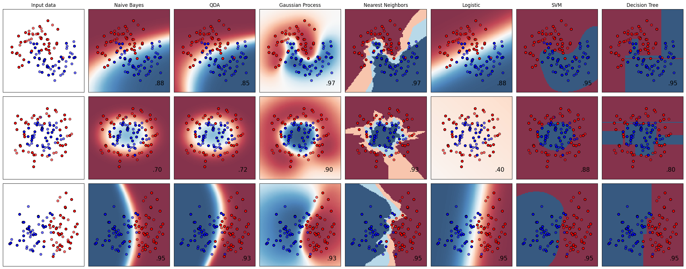
Part A Question: How does each of these methods generate the “probability”? Document your discussion in class below (just 1-2 sentences each). Note the name(s) of your group partner(s).
// Write your answer here
Gaussian Naive Bayes:
Discriminant Analysis:
Gaussian Process:
K-Nearest-Neighbor:
Logistic regression:
Support Vector Machine:
Decision Tree:
B. Decision Trees and Random Forests#
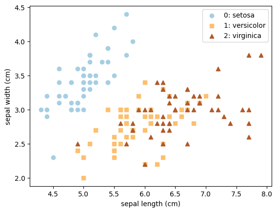
In this example, we still use the Iris data set. Like in Lab 14, because we are using the data set only as a demonstration, we will use all data as training data, so again be aware that this is not a good practice when you have a real problem to tackle!
import numpy as np
import matplotlib.pyplot as plt

from sklearn import datasets
from sklearn.tree import DecisionTreeClassifier, plot_tree
from sklearn.ensemble import RandomForestClassifier
from sklearn.model_selection import GridSearchCV
# Load and plot the iris data
iris = datasets.load_iris()
X = iris.data
Y = iris.target

n_classes = len(iris.target_names)
for i in range(n_classes):
    plt.scatter(X[Y==i, 0], X[Y==i, 1], color=plt.cm.Paired(i/(n_classes-1)), marker="os^"[i], label=f"{i}: {iris.target_names[i]}")
plt.legend()
plt.xlabel(iris.feature_names[0])
plt.ylabel(iris.feature_names[1]);
B1. Visualizing Trees#
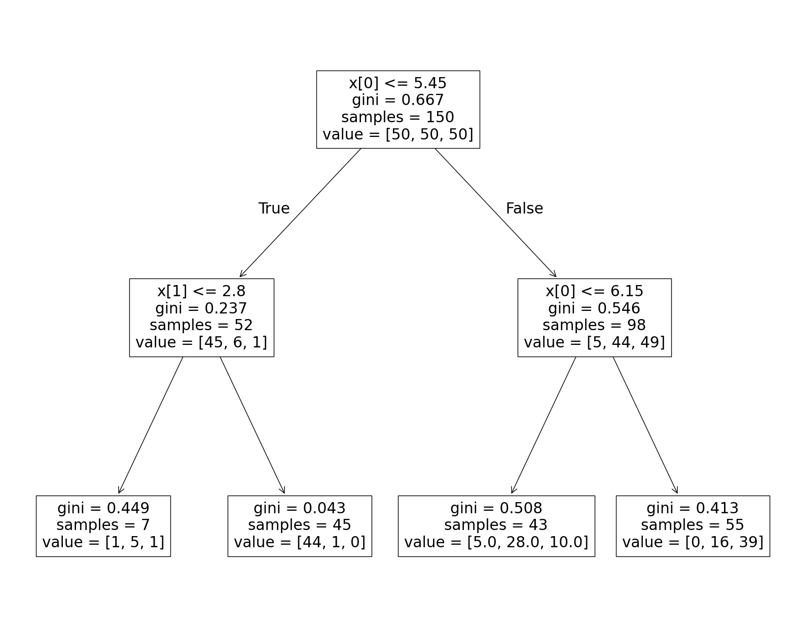
Here is the code that generates the tree diagram that we looked at together in class. You can use the plot above to inspect how the decision tree works (no written response needed).
clf = DecisionTreeClassifier(max_depth=2, criterion="gini")
clf.fit(X[:,:2], Y)

fig, ax = plt.subplots(figsize=(20, 16))
plot_tree(clf, ax=ax);
B2. Use cross validation to find tree depth#
Here we use the cross validation method (seen in Lab 13) to find the ideal tree depth for this data set, for both the decision tree and random forest methods.
tree_cv = GridSearchCV(DecisionTreeClassifier(), {"max_depth": np.arange(1, 11)})
tree_cv.fit(X, Y);
forest_cv = GridSearchCV(RandomForestClassifier(), {"max_depth": np.arange(1, 11)})
forest_cv.fit(X, Y);
plt.plot(tree_cv.cv_results_["param_max_depth"].data, tree_cv.cv_results_["mean_test_score"], '.-', label="tree")
plt.plot(forest_cv.cv_results_["param_max_depth"].data, forest_cv.cv_results_["mean_test_score"], 'x-', label="forest")
plt.legend()
plt.xlabel("max_depth")
plt.ylabel("mean test score");
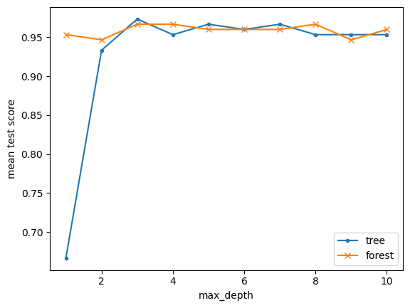
Part B2 Question: Based on the plot above, for this data set, what tree depth would you choose for the decision tree method and for the random forest method respectively?
// Write your answer here
C. Ensemble Methods#
This example shows how to use an ensemble method with scikit-learn! Complete the task and answer the question below (the main purpose is to get you familiar with scikit-learn API for ensemble methods).
Task: Add two more ensemble classifiers to the code (add to the classifiers list; keep the existing two). The specifications of the two classifiers are:
Adaptive boosting (
AdaBoostClassifier) with the Support Vector Machine Classifier (SVC) as the base estimator.Stacking method (
StackingClassifier) with the Logistic Regression (LogisticRegression), Quadratic Discriminant Analysis (QuadraticDiscriminantAnalysis), and Random Forest (RandomForestClassifier, use the depth you found in Part B) as the three base estimators.
from sklearn.ensemble import StackingClassifier, BaggingClassifier, AdaBoostClassifier, VotingClassifier

from sklearn.naive_bayes import GaussianNB
from sklearn.neighbors import KNeighborsClassifier
from sklearn.gaussian_process import GaussianProcessClassifier
from sklearn.tree import DecisionTreeClassifier
from sklearn.svm import SVC
from sklearn.discriminant_analysis import QuadraticDiscriminantAnalysis
from sklearn.linear_model import LogisticRegression
classifiers = [
    BaggingClassifier(KNeighborsClassifier(3), random_state=42),
    VotingClassifier([
        ("nb", GaussianNB()),
        ("gp", GaussianProcessClassifier(random_state=42)),
        ("knn", KNeighborsClassifier(3)),
        ("tree", DecisionTreeClassifier(max_depth=5)),
    ]),
    # TODO: add your code here
]

fig, ax = plt.subplots(1, len(classifiers), figsize=(4*len(classifiers),4))

for i, clf in enumerate(classifiers):
    clf.fit(X[:,:2], Y)
    DecisionBoundaryDisplay.from_estimator(
        clf,
        X[:,:2],
        cmap=plt.cm.Paired,
        ax=ax[i],
        response_method="predict",
        plot_method="pcolormesh",
        shading="auto",
        xlabel=iris.feature_names[0],
        ylabel=iris.feature_names[1],
    )
    ax[i].scatter(X[:, 0], X[:, 1], c=Y, edgecolors="k", cmap=plt.cm.Paired)
    ax[i].set_title(clf.__class__.__name__)
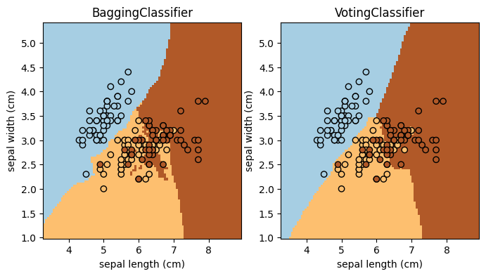
Part C Question: Which of these four methods (the two existing and the two you added) seems to work the best for this particular data set? Explain your reasoning in a few sentences.
// Write your answer here
Tip
How to submit this notebook on Canvas?
Make sure all your answers, code, and desired results are properly displayed in the notebook.
Save the notebook (press
Ctrl+sorCmd+s). The grey dot on the filename tab (indicating “unsaved”) should disappear.Run the following cell.
Upload the resulting HTML file to Canvas under the corresponding assignment.
! jupyter nbconvert --to html ./15.ipynb
